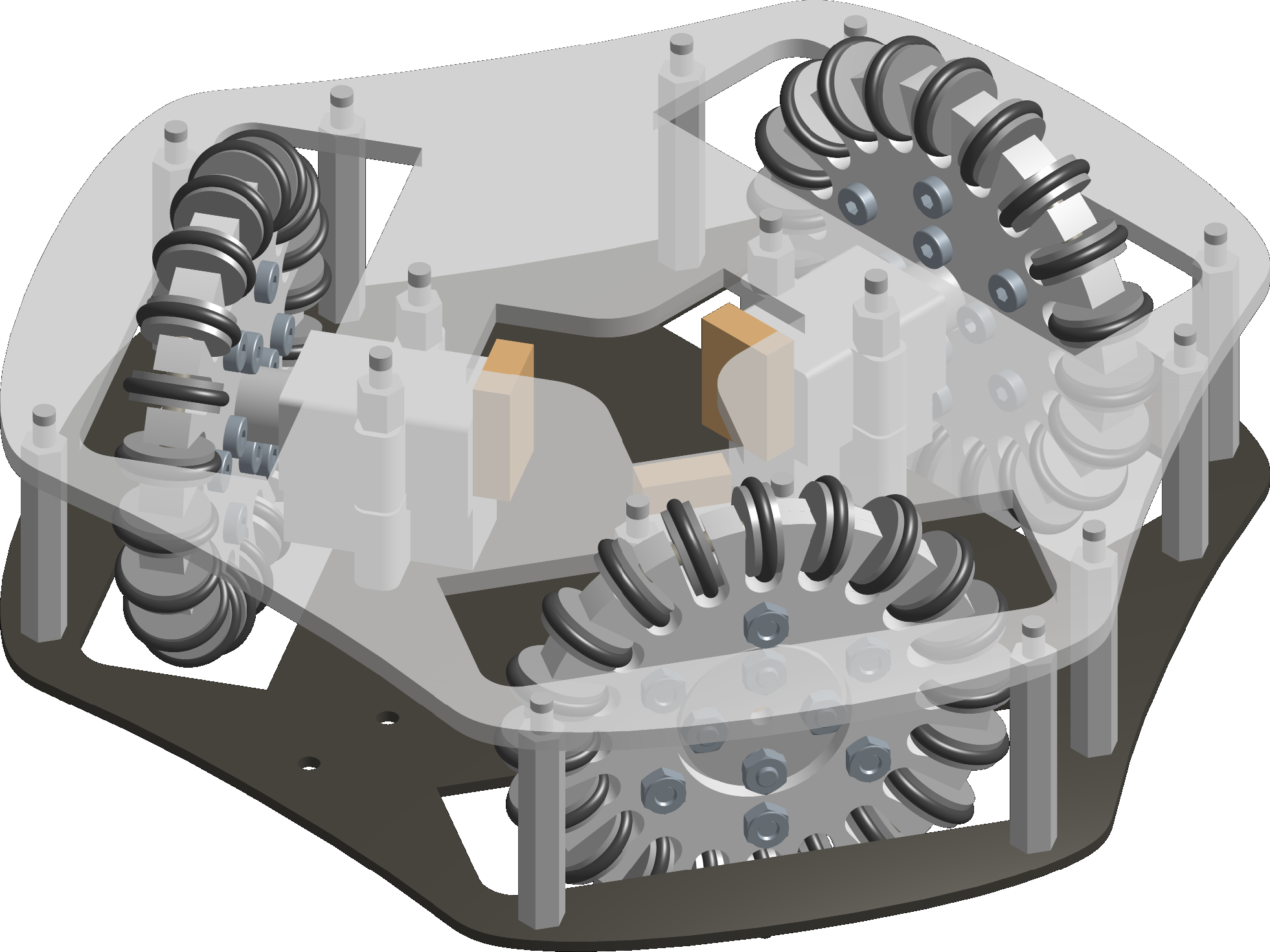
Kinematics of omni-directional wheeled robots

2022-10-30 #robotics #kinematics #omnidirectional #wheels

Omni-directional robots (sometime called holonomic robots) are platforms designed to allow a wide range of motion thanks to their wheels mechanically designed to allow lateral sliding motion. You can find such design in our open-source Robot Soccer Kit for instance.

Even if less intuitive than their differential (2-wheels) counterpart, the kinematics model of such platform is arguably easier to derive, and they are easier to control since the motion is less constrained. This is what we are going to explain in detail in this post.

Velocity

To focus on kinematics, we will consider the motors as sources of velocities. The very first question we might ask is: what are the nature of velocities our robot could possibly achieve?

The velocity of an object can be described with the velocity of all its particles. However, our robot is a rigid body, which means that its particles are staying at the same distance relative to each other.

Transformations preserving those distances are translations and rotations. In the plane, a translation summed with a rotation yields a rotation about another center, thus, pure translation and rotation about an arbitrary center are the only possible motions. For instance, here are the velocities of particles attached to the rigid body of the robot while it rotates about the blue point:

What we see here is a field of vectors describing the velocities of points attached to the rigid body of the robot. Note that these points can be immaterial (they are not necessarily part of the robot, but they move with its body).

Core tools

Before we go any further, we will remind basic tools that are important to derive robot kinematics.

Cross product

First, let’s define an axis of rotation \(\vec \omega\) as a vector which orientation indicates us about which axis we are rotating, and which norm is the velocity of rotation (in rad/s).

Suppose a point \(P\) rotates around this axis, and we know some point \(O\) belonging to the axis (thus, its velocity caused by the rotation is zero). Here, the so-called vectorial cross product, denoted \(\vec \omega \times \vec{OP}\) gives us the velocity of the point \(P\):

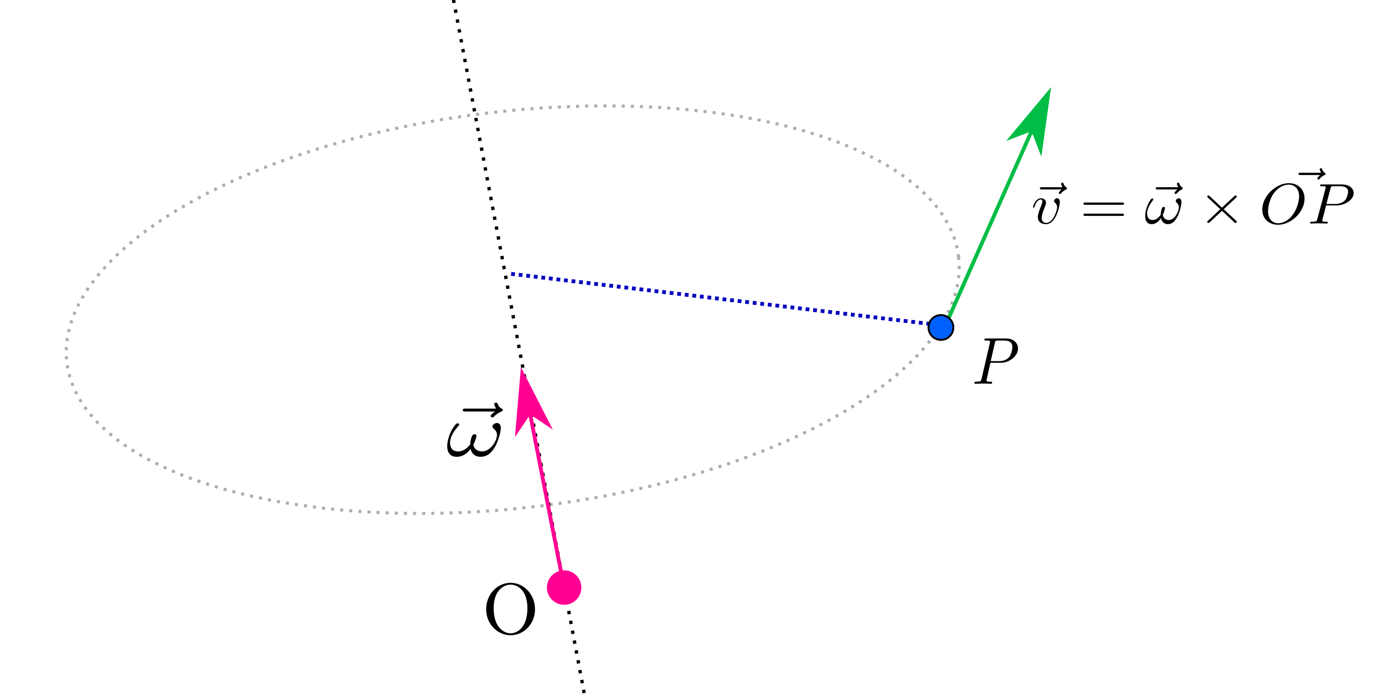
This cross product can be computed as:

\[\begin{bmatrix} \omega_x \\ \omega_y \\ \omega_z \end{bmatrix} \times \begin{bmatrix} p_x \\ p_y \\ p_z \end{bmatrix} = \begin{bmatrix} \omega_y p_z - \omega_z p_y \\ \omega_z p_x - \omega_x p_z \\ \omega_x p_y - \omega_y p_x \end{bmatrix}\]

We can show that this operation is distributive over addition.

Varignon’s formula

If we now have two points \(P_1\) and \(P_2\), we can deduce their velocities \(\vec v_1\) and \(\vec v_2\) the same way:

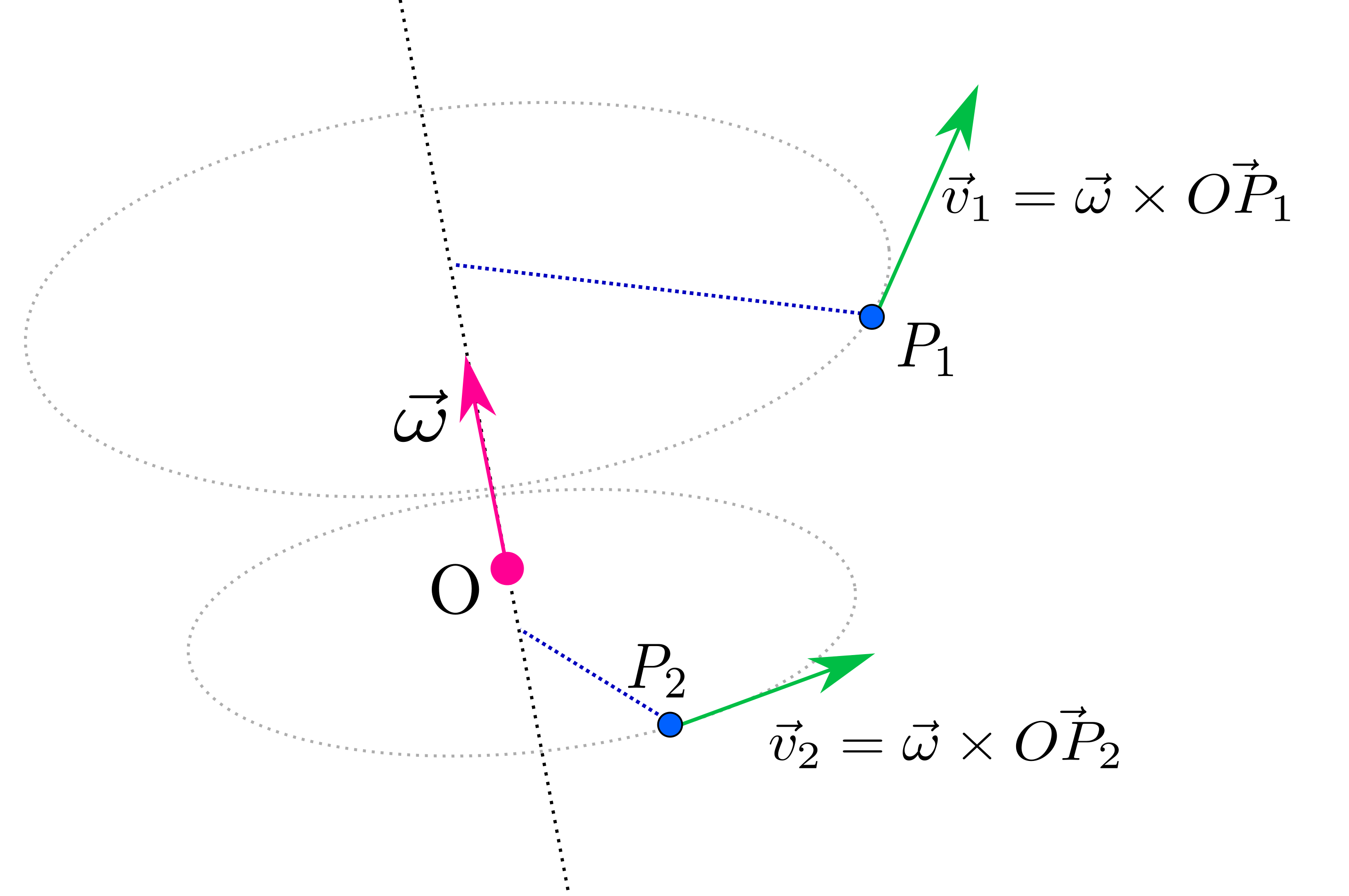
And, thus:

\[\begin{array}{l} \vec v_2 = \vec \omega \times \vec {OP_2} \\ \vec v_2 = \vec \omega \times (\vec {OP_1} + \vec {P_1 P_2}) \\ \vec v_2 = \vec \omega \times \vec {OP_1} + \vec \omega \times \vec {P_1 P_2} \\ \vec v_2 = \vec v_1 + \vec \omega \times \vec {P_1 P_2} \end{array}\]

In other words, if we know the velocity \(\vec v_1\) of a particular point \(P_1\) and the velocity of rotation \(\vec \omega\), we can deduce the velocity of any other point \(P_2\) using the relation \(\vec v_2 = \vec v_1 + \vec \omega \times \vec {P_1 P_2}\). The whole vector field mentioned before is totally known. In particular, the need of a known point belonging to the rotation axis vanishes.

This equation is sometime refereed to as Varignon’s formula. This result is a core tool of screw theory which is extensively based on this transformation.

You can also notice that this also works for pure translations: since the cross product will be zero, the velocity will be the same for all points.

Kinematics model

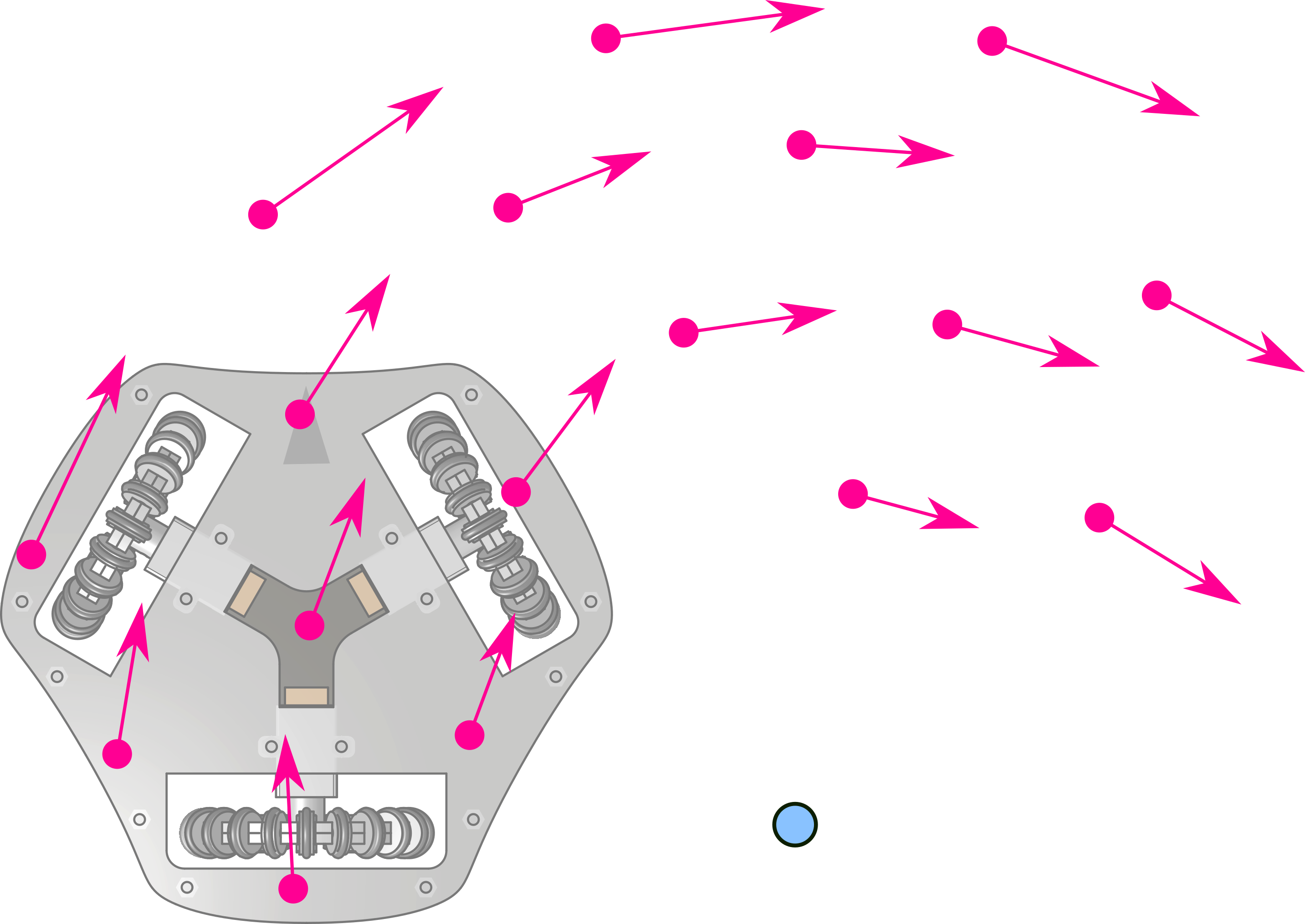
Robot’s geometry

When we build our robot, we know its geometry, it can be parametrized using the following values:

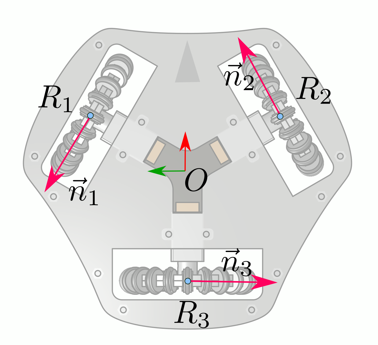
Here:

We chose a reference frame attached to the robot chassis, placed at the center, with the \(x\) axis forward and \(y\) axis on the left (\(z\) axis would be upward). Later, when we will give a velocity target, we will express it in this frame,
The points \(R_i\) are the position of the wheels,
The vectors \(\vec n_i\) are the drive vectors for the wheels. They are oriented toward where the wheel is going to turn and drive. Since they are of unit length, they can be parameterized using only one number (like an angle with the x-axis).

Deriving wheel velocities

We’ll start with our desired velocity, that we will express in the chassis frame:

\[s = \begin{bmatrix} \dot x \\ \dot y \\ \dot \theta \end{bmatrix}\]

In 3D, our goal is to reach the following chassis velocity (expressed in the robot frame):

\[\begin{matrix} v_o = \begin{bmatrix} \dot x \\ \dot y \\ 0 \end{bmatrix} & \omega = \begin{bmatrix} 0 \\ 0 \\ \dot \theta \end{bmatrix} \end{matrix}\]

With \(v_o\) being the velocity of the robot’s origin and \(\omega\) the robot’s rotation velocity. The zeros are here because we are in 3D (the robot is not moving upward and is not tilting forward or laterally).

Thanks to Varignon’s formula, we can now express the resulting velocity in the wheels:

\[\begin{array}{l} \vec v_i = \vec v_o + \vec \omega \times \vec{OR_i} \\ v_i = \begin{bmatrix} \dot x - y_i \dot \theta \\ \dot y + x_i \dot \theta \\ 0 \end{bmatrix} \end{array}\]

Where \(x_i\) and \(y_i\) are the coordinates of \(\vec{OR_i}\) in the robot frame.

We can now compute \(w_i\), the component of this velocity that is in the direction of the wheel, using the dot product with its drive vector:

\[\begin{array}{l} w_i = \vec{v_i} \cdot \vec{n_i} \\ w_i = {n_i}_x (\dot x - y_i \dot \theta) + {n_i}_y (\dot y + x_i \dot \theta) \\ w_i = {n_i}_x \dot x + {n_i}_y \dot y + ({n_i}_y x_i - {n_i}_x y_i) \dot \theta \end{array}\]

We obtain a linear relation between the target (chassis) velocity and the linear velocity of a wheel.

Note that \(w_i\) is linear velocity expressed in m/s, we still need to divide it with our wheel radius if we want a rotation velocity expressed in rad/s.

Matrix notation

Since everything is linear, we can then express the velocity of our wheels as a linear transformation of the desired chassis velocity:

\[\underbrace{ \begin{bmatrix} w_1 \\ w_2 \\ w_3 \end{bmatrix} }_w = \underbrace{ \begin{bmatrix} {n_1}_x & {n_1}_y & ({n_1}_y x_1 - {n_1}_x y_1) \\ {n_2}_x & {n_2}_y & ({n_2}_y x_2 - {n_2}_x y_2) \\ {n_3}_x & {n_3}_y & ({n_3}_y x_3 - {n_3}_x y_3) \end{bmatrix} }_M \underbrace{ \begin{bmatrix} \dot x \\ \dot y \\ \dot \theta \end{bmatrix} }_s\]

Note: if the motor drive direction is perpendicular to the position of the wheel, then \(M\) can be simplified to:

\[\begin{bmatrix} {n_1}_x & {n_1}_y & d \\ {n_2}_x & {n_2}_y & d \\ {n_3}_x & {n_3}_y & d \end{bmatrix}\]

Where \(d\) is the distance between the wheels and the center of the robot.

Direct kinematics

If \(M\) has a full rank, it can be inverted to deduce the chassis velocity from the wheels velocity:

\[s = M^{-1} w\]

This is the direct kinematics model. It can be used to compute the odometry of the robot for instance.

Velocity limits

One way to model the motors physical limitations is to consider that they can provide velocities under a given maximum limit, say \(w_{max}\).

If we don’t take care of this limit, and increase a target velocity \(s\), we will first saturate the velocity of one motor (say \(w_1\)), and the velocity of other motors will continue to rise. This will have the effect of getting the robot to move in a different direction than the one initially desired.

Another approach would be to “rescale” \(w\) so that none \(|w_i|\) would be greater than \(w_{max}\). For instance, if \(w_1 > w_{max}\) and is the biggest wheel velocity, then, we can use \(w' = \lambda w\) as target velocity for wheels, with \(\lambda = \frac{w_{max}}{w_1}\).

This approach is valid because \(w = Ms\) is a linear relation, then \(\lambda w = M (\lambda s)\). Hence, rescaling \(w\) is equivalent to rescale \(s\) (the direction of the target in task space is preserved).

A geometrical view of velocity limits

Another way to view the limits is to think them as a set of inequalities:

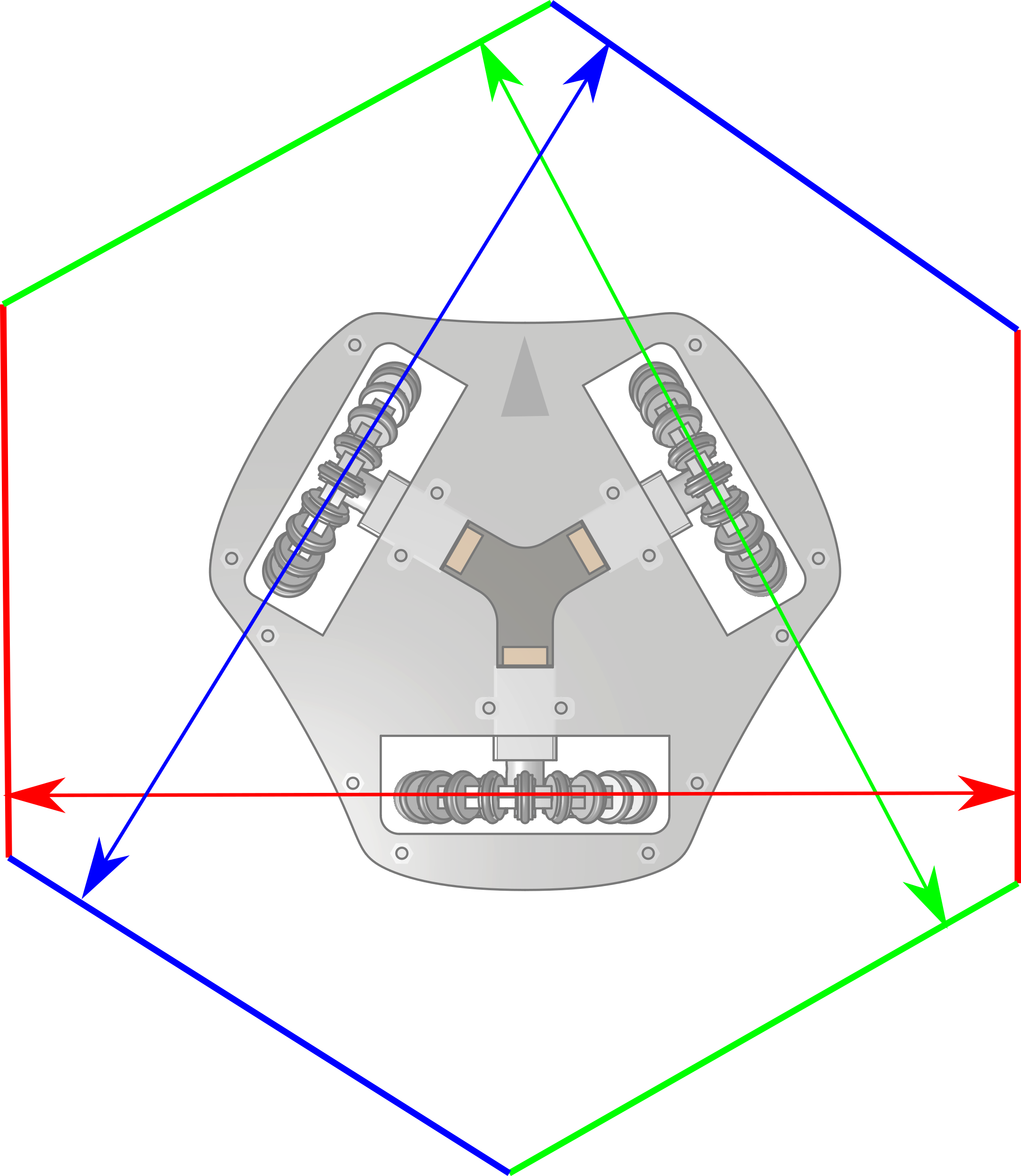
\[|w| \leq w_{max}\]

Such equations defines what we call a polytope, which is a particular type of 3D shapes. In this case, the shape is simply a cube. If we now express this constraint in terms of task space, we get:

\[|Ms| \leq w_{max}\]

Here, since everything is linear, \(M\) will scale and tilt the original cube. Here is the result for a robot with three wheels dispatched evenly at 120° (like the figures above):

Any point in this new shape is a valid velocity in the task space (a target velocity giving feasible wheel velocities). If we slice this cube where \(\dot \theta = 0\), we can visualize what velocities are possible to achieve when no rotation is involved (the violet area below):

You can notice that the cube gets here sliced to an hexagon (I personally finds this geometrical detail elegant, but it’s up to your taste!).

As you can notice, the robot velocity capabilities are not the same in all the directions. Actually, if you notice that velocity limits are reached when the target velocity is collinear with a wheel, you can intuite this hexagon: