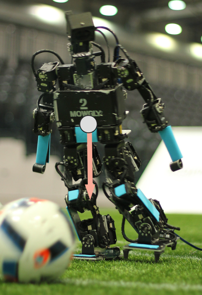
As opposed to robotic arms, humanoid robots are mobile and therefore contact points with the environment should be accounted for when computing their dynamics.
Here, we derive a way to compute the required torque on a humanoid robot standing on either one or two legs to sustain gravity.
Introduction
The general equation of motion is:
\[M(q) \dot v + g(q) + h(q, v) = \tau \space \space (1)\]Where:
- \(q\) is the configuration of the robot joints,
- \(v\) is the speeds of the robot joints (and \(\dot v\)) acceleration of robot joints,
- \(M(q)\) is the mass matrix,
- \(h(q, v)\) are Coriolis and centripetal effects,
- \(g(q)\) is the generalized gravity,
- \(\tau\) are the degrees of freedom torque.
For a static position, velocity \(v\) and acceleration \(\dot v\) are zero, and the equation becomes:
\[\tau = g(q)\](Note that \(h\) vanishes when \(v\) is zero).
Thus, for any “static” robot like a robotic arm anchored to the ground, we can simply stop here. The generalized gravity is indeed directly the joint torques we need to compensate gravity.
Floating base
Now, what if we have a mobile robot, like a humanoid? The thing is that we need to represent the fact that the robot is moving in the world. This is typically achieved by adding a floating base.
The floating base is a set of 6 extra degrees of freedom added at the beginning of the kinematics chain representing the position of the robot in the world.
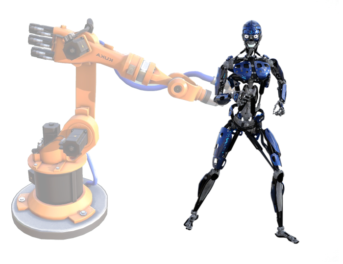
As an illustration, imagine an humanoid robot attached to an invisible robotic arm itself anchored to the ground. (This is just a mental visualization; the floating base is of course not constrained to the singluarities and the workspace of a robotic arm).
Equation \((1)\) now becomes:
\[M(q) \dot v + g(q) + h(q, v) = \begin{bmatrix} 0_6 \\ \tau \end{bmatrix}\]Where \(0_6\) is the dimension-\(6\) vector of zero torques in the floating base. Subject to gravity, the only way to balance this equation is to include some acceleration on the floating base: the robot is “falling” and there is no way to prevent that because our current model doesn’t includes contact forces.
Contact forces
Contact forces act on the robot through the transpose of the contact frame Jacobian. For more information see Modern Robotics, chapter 5.2.
Those additional terms can be added to equation \((1)\), which is now:
\[M(q) \dot v + g(q) + h(q, v) = \begin{bmatrix} 0_6 \\ \tau \end{bmatrix} + \underbrace{ \sum_i J_i^T f_i }_{contact forces} \space \space (2)\]Again, assuming we want no acceleration and neglecting other non linear effects than gravity, our equation becomes:
\[g(q) = \begin{bmatrix} 0_6 \\ \tau \end{bmatrix} + \sum_i J_i^T f_i \space \space (3)\]One support leg
With one support leg, equation \((3)\) now is:
\[g(q) = \begin{bmatrix} 0_6 \\ \tau \end{bmatrix} + J_l^T f_l\]Where \(J_l\) is the Jacobian of the left foot and \(f_l\) the wrench (a 6D vector packaging the forces and their moments) applied on the left foot.
We can split this equation in two parts:
\[\begin{cases} g_u(q) = (J_l^T)_u f_l \\ g_a(q) = \tau + (J_l^T)_a f_l \end{cases}\]Here, the subscripts \(u\) and \(a\) denote respectively the unactuated and actuated parts of the gravity and Jacobian.
Since \((J_l^T)_u\) is the Jacobian of an universal floating base, it can always be inverted, and:
\[f_l = (J_l^T)_u^{-1} g_u(q)\]Is the only solution of contact forces to balance the equation. We can then substitute them back in the actuated part of equation and get:
\[\tau = g_a(q) - (J_l^T)_a (J_l^T)_u^{-1} g_u(q)\]Which are the torques needed on the robot joints.
Two support legs
We now assume two support legs, and then have:
\[g(q) = \begin{bmatrix} 0_6 \\ \tau \end{bmatrix} + J_l^T f_l + J_r^T f_r\]With \(J_l\) and \(J_r\) being respectively the Jacobian of the left and right foot, and \(f_l\) and \(f_r\) respectively the contact wrenches on the left and right foot.
We can do the same split as previously, but separating also equations for left and right legs:
\[\begin{cases} g_u(q) = (J_l^T)_u f_l + (J_r^T)_u f_r \space \space (4) \\ g_l(q) = \tau_l + (J_l^T)_l f_l + \underbrace{(J_r^T)_l}_0 f_r \space \space (5) \\ g_r(q) = \tau_r + \underbrace{(J_l^T)_r}_0 f_l + (J_r^T)_r f_r \space \space (6) \end{cases}\]Because of the kinematics structure of the robot, we know that \((J_r^T)_l\) and \((J_l^T)_r\) are zero (because left and right legs are different branches in the kinematics tree).
Here, we can’t solve contact forces using the first equation, because the system is under-constrained. Indeed, forces have 12 degrees of freedom while we only have 6 equations.
Minimizing contact forces
We could solve equation \((4)\) with:
\[\begin{bmatrix} f_l \\ f_r \end{bmatrix} = \begin{bmatrix} (J_l^T)_u & (J_r^T)_u \end{bmatrix}^{\dagger} g_u(q)\]Where \(\dagger\) denotes the Moore-Penrose pseudo-inverse. (Note: With Numpy, you can use np.linalg.pinv, and with Eigen you can use computeOrthogonalDecomposition().solve().)
That would give us the solution that minimizes contact forces (more precisely \(|| f_l ||^2 + || f_r ||^2\)). But if you want to control a humanoid robot, it is more likely that what you want to minimize is the torques used in the motors instead.
Minimizing torques
We can turn equation \((4)\) into a relation between \(f_l\) and \(f_r\):
\[f_l = \underbrace{ - (J_l^T)_u^{-1} (J_r^T)_u }_A f_r + \underbrace{ (J_l^T)_u^{-1} g_u(q) }_B\]Substituing it in \((5)\), we get:
\[(J_l^T)_l f_l = g_l(q) - \tau_l \\ (J_l^T)_l (A f_r + B) = g_l(q) - \tau_l \\ f_r = \underbrace{ - ((J_l^T)_l A)^{-1} }_C \tau_l + \underbrace{ ((J_l^T)_l A)^{-1} ( g_l(q) - (J_l^T)_l B ) }_D \space \space (7)\]And, from \((6)\):
\[f_r = \underbrace{ - (J_r^T)_r^{-1} }_E \tau_r + \underbrace{ (J_r^T)_r^{-1} g_r(q) }_F \space \space (8)\]Thus, combining \((7)\) and \((8)\), we can get a relation between \(\tau_l\) and \(\tau_r\):
\[C \tau_l + D = E \tau_r + F\]Which is another under-constrained system expressed in terms of torques. We can now find the solution minimizing torques:
\[\begin{bmatrix} \tau_l \\ \tau_r \end{bmatrix} = \begin{bmatrix} C & -E \end{bmatrix}^{\dagger} (F-D)\]It is not over
It seems that we now have a solution to the initial problem. However, we forgot a strong assumption: contact forces are unilateral. This means that we can’t “pull” on the ground for example.
The solution to the single support foot equation is unique, thus, while we can check if it is feasible, there are no other torques we could apply. However, the solution with two support feet is under-constrained and admits an infinite set of solutions.
What we want is to explore those solutions, and select the one that minimizes torques subject to some constraints on the force (in that case, \(f_z > 0\), if \(f_z\) is expressed in the proper frame).
To achieve this, we can formulate the problem as a quadratic programming (QP) problem and invoke a solver. Such a solver can address problems of the form:
\[min_x \space \frac{1}{2} x^T P x + c^T x \\ subject \space to: \\ A x = b \\ G x \leq h\]Let’s consider the double support problem here. As you will see, this formulation can also be easily extended to any number of contact forces.
Optimization variables
The optimization variables that we will use are:
\[x = \begin{bmatrix} \tau_a & f_l & f_r \end{bmatrix} ^T\]Where \(\tau_a\) is the robot torques, and where \(f_l\) and \(f_r\) the contact forces.
Objective function
To define our score function, we will choose \(c\) to be 0, and \(P\) to be a diagonal matrix, with \(1\) on the diagonal for values that correspond to an actuated torque, and \(\epsilon\) for contact forces.
If you think about it, with this \(P\), the resulting score will be the sum of the (squared) torques, plus the sum of the (squared) forces times \(\epsilon\). This means that the main priority is to find the solution with the minimum torques, and the second priority (with a very small weight) is to minimize contact forces.
This trick is required since the forces are part of our optimization variables and the QP solver needs a score to be minimized for all those variables.
Equality constraint
The equality constraint is the one we’ve been dealing with the whole time:
\[\underbrace{ \begin{bmatrix} 0 & (J_l^T)_u & (J_r^T)_u \\ I & (J_l^T)_a & (J_r^T)_a \end{bmatrix} }_A \begin{bmatrix} \tau \\ f_l \\ f_r \end{bmatrix} = \underbrace{ g }_b\]Here, again, \(u\) and \(a\) subscript refers to unactuated and actuated parts of the jacobian.
Inequality constraint
The problem we formulated so far is already a quadratic program, and does exactly what was explained in detail in the previous section, but in a cleaner way.
We can now take advantage of quadratic programming’s real advantage, inequality constraints, to ensure that our contacts are unilateral:
\[f_{l_z} \geq 0 \\ f_{r_z} \geq 0\]Those constraints can be set by adding two rows in \(G\) and \(h\).
\[\underbrace{ \begin{bmatrix} ...0... & -1 & ...0... & 0 & ...0... \\ ...0... & 0 & ...0... & -1 & ...0... \end{bmatrix} }_G \begin{bmatrix} ... \\ f_{l_z} \\ ... \\ f_{r_z} \\ ... \end{bmatrix} \leq \underbrace{ \begin{bmatrix} 0 \\ 0 \end{bmatrix} }_h\]In practice
In practice, you can consider using:
- Python: qpsolvers
- C++: Eiquadprog
But there are many other implementations and libraries out there!
More generally
Solving tasks-space problem with dynamics using QP solvers is extensively studied in robotics.
This is what is achieved in solvers like TSID (Task-Space Inverse Dynamics). In such setup, you minimize a score function subject to equation \((2)\), using some solver like Quadratic Programming.
Thanks to Stéphane Caron and Marcos Maximo for proof-reading, comments and typos feedbacks.
 Gregwar
 @greg_war